The poll-averaging model I've developed for HuffPost generates estimates of Obama and Romney vote share in each state, and for the national level popular vote. The model also produces probabilities of an Obama lead in each state and in the national popular vote.
As we enter the final week of the campaign, an obvious question to ask is how to convert the state-by-state probabilities of an Obama or Romney lead in the polls to probabilities that Obama or Romney will win the state and the election itself.
A key element of the model is that it makes corrections for house effects, the tendency of a given pollster to produce numbers that systematically lean towards one candidate (or party). Over the course of the campaign I've hardwired a key constraint into the model; that looking over all the survey houses in the HuffPost/Pollster data base, the average house effect is zero. In other words, averaged over survey houses, the polls "get it right," or at least that is a key assumption of the poll-averaging model I developed for HuffPost.
If this is wrong -- say, if the polls are collectively underestimating Romney support -- then the house effects distribution needs to shift up from the assumed mean of zero (i.e., there is more pro-Obama bias across pollsters than I've been assuming); on the other hand, if the polls are collectively under-estimating Obama support, then the house effects distribution needs to shift down from the assumed mean of zero (there is more pro-Romney bias across pollsters than I've been assuming).
For the purposes of converting the poll average to a forecast, I'll now relax the assumption that the polls are collectively unbiased. Assuming that house effects average to zero might make sense when we're averaging the polls. But for forecasting, we need to confront an extra source of potential bias and variability. In particular, the polling industry might not "get it right" averaged over the survey houses in the Pollster database.
Past elections give us some guide to how poll averages have missed actual election outcomes. Bob Erikson and Chris Wlezien's Timeline of Presidential Elections presents some summaries of the relevant data, using data from 1952 to 2008. John Sides' paraphrase of the key Erikson and Wlezien finding:
In very close elections, the polls are still quite close to the actual outcome -- missing by 1-2 points at most.
Nate Silver at FiveThirtyEight published a list of pre-election poll averages and actual outcomes from 1972 to 2008. This isn't a lot of data on which to base a mapping from poll averages to election outcomes; indeed, the 1972 poll "average" is based on just one poll, but there are 24 polls contributing to the (very accurate) 2008 poll average. Changes in technology in the polling industry (e.g., cell phones vs landlines, robo-polling, Internet panels) mean that we should probably give more recent years greater weight than earlier years in assessing the relevance of the historical data on this question.
At the same time, we also want to protect against outliers or "rare events" (or, if you prefer, the polling industry's version of a "Black Swan"). That is, precisely because we have relatively little data to work with, we don't want to rule out the possibility that the polls could be quite wrong. For this reason I fit a "heavy-tailed" distribution to the historical data (again, see the technical notes, below, for an explanation).
Finally, I don't want to replace the somewhat restrictive "average house effect is zero" assumption with an alternative assumption that is similarly restrictive, say, the "average house effect is 0.5 percent." Rather, I adopt an approach that concedes that we simply don't know with certainty what the error of the poll average will be; I use a (heavy-tailed) probability distribution to characterize my uncertainty over the error of the poll average. Analysis of the temporally discounted, historical data supplies information as to the shape and location of that distribution.
Details appear below, but the key idea is that I will replace the "average house effect is zero" assumption with an assumption that says in the average election, the average house effect is zero, but there is substantial election-to-election variation in how well the polls perform. In any given election, the average house effect could be smaller or larger (the polls could collectively favor one candidate or the other and by smaller or larger amounts). Our problem is that we don't know what type of election we've got (at least not yet). We should buy some insurance when we move from poll averaging to talking about state-level predictions, with some uncertainty coming into our predictions via uncertainty over the bias of the poll average we might encounter this cycle.
This extra uncertainty is not insubstantial, and trims the confidence with which we think either candidate is ahead in key swing states, "shrinking" the probabilities towards 50 percent, as shown in the following table, based on analysis of the Pollster data base as it looked late last night (10/29/12):
The polls have been quite unequivocal in pointing to Obama leads in Ohio, Nevada, Wisconsin and Iowa; my model-based poll average has been estimating the probabilities of Obama poll leads there at above 90 percent and even above 95 percent in some cases. Ohio has seen much polling, and my poll average there has consistently had Obama leading with high confidence. Once we factor in uncertainty about the average bias of the polls (or equivalently, where to center the house effects distribution) -- effectively converting a pre-election poll average into a forecast of sorts -- this Obama lead probability falls from 97 percent to an "Obama win" probability of 71 percent.
In New Hampshire, Obama's "poll lead" probability of 82 percent falls to a 63 percent "win" probability. In Virginia and Colorado, the corresponding probabilities are 75 percent and 59 percent. On the side of the ledger, Florida moves only a little, from a 40 percent "Obama poll lead" probability to a 45 percent "Obama win" probability, and North Carolina moves from 11 percent to 32 percent.
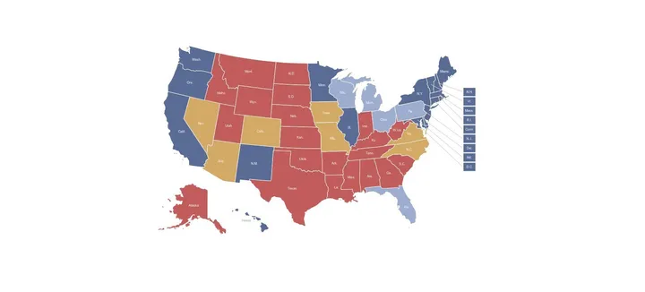
And yes, in the midst of this technical discussion it is worth noting that of the nine states considered here, only two are leaning towards Romney: Florida and North Carolina.
The national popular vote also moves towards a 50 percent probability once we engage in the same exercise, translating the probability of a poll average lead into the probability of a win in the election. My model has been generating estimates of the national popular vote that have been delicately poised of late. Romney has been recording a small lead in the national level poll average in recent weeks, of anywhere between 0.2 to 0.6 percentage points. Even with the large volume of national polling, the difference between Obama and Romney national poll averages is so small that we can't confidently say Romney leads Obama or vice-versa; at the time of writing, the probability that Obama leads Romney is just 39 percent, at least according to my model-based poll average. [An aside: this probability can drift up to suggest it is more likely that Obama leads Romney, depending on the precise mix of polls in the analysis on any given day, a point I'll elaborate between now and Election Day.] But when we acknowledge uncertainty in the average house effect, the national popular vote story is effectively 50-50.
Finally, the Electoral College picture. Because my model-based poll averaging generates such precise estimates at the state level, the implied Electoral College picture has been confidently pointing to an Obama lead. With extremely high probabilities of Obama poll leads in most swing states, the implied probability of a lead in the Electoral College has been north of 95 percent since the Democratic convention, and even after the first debate. Uncertainty as to the average house effect correction -- something we need to take into account as we pivot from poll average to election forecast -- tempers this estimate, shifting the probability of an Obama win into the low 70 percent region.
I stress that the overall picture is not wildly dissimilar under the two sets of modeling assumptions: i.e., we're looking at an extremely close national vote, but swing state polling continues to point to an Obama win in the Electoral College, and perhaps even a comfortable win in the Electoral College at that.
Finally, if I were to engage in some fine-tuning of these estimates, I'd shade them in the direction of the poll averages. If anything, the model I fit to generate a distribution over the house effects is perhaps too permissive, too cautious. The heavy-tailed model I employ here contemplates a much worse performance by the polls than that found by Erikson and Wlezien, at least in close elections. If we were to simply take the Sides paraphrase of Erikson and Wlezien -- that in close elections, the polls are never off by more than 1 or 2 points -- then the trimming of the "poll lead" probabilities reported above would be less dramatic.
Technical notes: We have a small data set of poll averages, taken from Nate Silver's table. The data are reproduced here. The two outliers in the data set are 1980 and 1996.
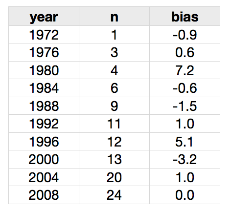
I apply two sets of weights to this small set of data: (1) a temporal discount factor, via a series of geometrically declining weights, with decay parameter 0.8 such that the 2008 data point gets weight 1, 2004 gets weight 0.8, 2000 gets weight 0.64; this was chosen after trial-and-error, but the results don't seem too sensitive to the precise choice; (2) the number of observations in each poll average. The product of these two weighting factors enters the modeling as the relative precision of each observation. The most recent observation is 2008 and has 24 polls in the poll average gets a "relative precision" of 24; the most temporally distant observation is 1972 and has just one observation and has a relative precision of .13. I readily concede that this weighting scheme is rather arbitrary.
I fit a t distribution to the weighted data with unknown mean, scale and degrees of freedom parameters; for small values of the degrees of freedom parameter (say, less than 30), the t distribution has heavier tails than the normal. I use Bayesian methods for this exercise, recovering posterior densities over the three parameters in the model. Point estimates (means of the marginal posterior densities) are: mean .36 (95 percent CI: -.94 to 1.7), scale .57 (95 percent CI: .11 to 2.3) and degrees of freedom 11.3 (1.2 to 28.8). That is, these data suggest very little evidence of systematic partisan bias in the poll averages, but a good deal of election-to-election variability in the fit of the poll averages to actual election outcomes. Indeed, there is substantial posterior probability mass on low degrees of freedom, indicating that the distribution that best fit to these (weighted) data is quite heavy-tailed.
I sample from this fitted model many times and store the results, building up a (Monte Carlo) approximation to the predictive distribution as to the bias of a poll average for a contemporary U.S. presidential election. This predictive distribution has the same mean as the fitted mean, .36 percentage points, but a 95 percent confidence interval that ranges from -4.4 to 5.3 percentage points; because this density is heavy-tailed, the 50 percent confidence interval is much smaller, ranging from about -0.9 to 1.6 percentage points. This uncertainty over the bias of a poll average is roughly in line with Sides' paraphrase of the Erikson and Wlezien analysis of "1 to 2 points", but with substantially larger biases also considered likely. I center this predictive distribution at zero; the small amount of Democratic bias suggested by the analysis is swamped by the uncertainty around the estimate, and shouldn't be taken too seriously given the arbitrary weighting scheme I applied to these data. The key point is that we have a plausible model for characterizing and generating uncertainty over the bias of the poll average.
So now, instead of the house effects "averaging to zero," I now re-run my poll averaging model subject to the constraint that the house effects sum to a quantity following the predictive distribution just described. Uncertainty as to the center of the house effects distribution induces uncertainty as to Obama and Romney vote shares and in turn, uncertainty over the Electoral College outcome, in addition to the other sources of uncertainty in the model (sampling variation in the polls, house effects, the magnitude of temporal drift in voter sentiment over the campaign, how much state and national estimates ought to influence one another, etc.).
Finally, some details on the last step of the computation. I use Monte Carlo simulation to convert the state-by-state probabilities of an Obama lead into an Electoral College count and the probability of an Obama victory. A simple way to do this is to use the probabilities produced by model and Monte Carlo simulation. That is, perform the following steps many times (typically, about 10,000 in each run of my model):
- For each state, flip a coin with probability of "heads" equal to the probability that Obama leads in that state.
- If the coin comes up heads, allocate that state's Electoral College votes to Obama (ignoring the possibility of a split allocation of Electoral College votes in Maine and Nebraska).
- Sum the Electoral College vote over states.
We note the proportion of times that Obama is allocated 270 Electoral College votes or more over many repetitions of this process. We report this quantity as the probability that Obama wins the election.