
The graph below shows point estimates of the survey house effects produced by my model (as of the evening of October 23, 2012). Negative house effects means that the pollster skews in a pro-Romney direction; positive house effects means that the pollster tends to overstate support for Obama.
The pollsters listed here are the more prolific and/or prominent pollsters appearing in the Pollster data base. The reported house effects are for the likely voter polls produced by these pollsters. The house effects are estimated subject to the assumption that the house effects have zero mean across the pollsters in the Pollster data base; that is, averaged across pollsters, the polls "get it right." That is, the house effects are best thought of as offsets relative to the industry-wide mean. The house effects are re-estimated with every new run of the model (every couple of hours).
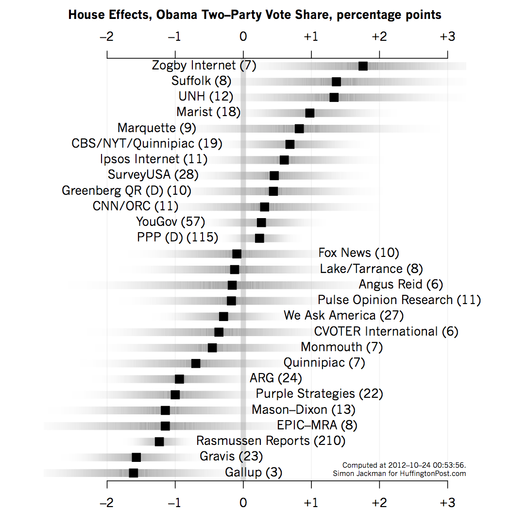
Each row of the graph shows an estimated house effect (solid square) in two-party terms; i.e., the Obama/(Obama + Romney) percentage, not the "raw" Obama percentage reported by any particular poll. The shaded bars convey a sense of the uncertainty around each estimated house effect, roughly extending out to cover a MOE (actually, a 95 percent credible interval). The number in parentheses after each pollster's name is the number of polls we have for each pollster in the HuffPost/Pollster database as of the time of writing.
Regular poll watchers will not be surprised by the findings here. The most prolific pollster in the Pollster data base -- Rasmussen -- tends to produce estimates that lean in a Republican direction. The model-based estimate of this bias about 1.2 points in two-party terms. Because Rasmussen polls so much, we learn about their house effect: a 95 percent credible interval (or MOE) around the estimated 1.2 point bias ranges from -1.6 to -0.9, well away from zero.
We have just a handful of Gallup LV polls; Gallup is reporting a week's worth of polling each day, and the HuffPost database only outputs the most recent series of non-overlapping polls for each run of the model. Thus, as of the time of writing, just 3 Gallup LV polls were available for analysis. Gallup has been producing estimate of the vote share starkly at odds with the rest of the industry, which manifests in an estimated house effect of -1.6 percentage points (in two-party terms) and with a large 95 percent credible interval ranging from -2.7 to -0.5. That is, if the industry consensus was 50-50 (Obama-Romney), we could expect Gallup to produce 48.4-51.6 results.
This is the largest house effect of any major pollster in the data base, 25 percent larger than the Rasmussen house effect. Mason-Dixon also appears to generate a sizeable pro-Romney house effect, as does Purple Strategies and ARG, around about a point of two-party vote share.
On the other side of the ledger, Zogby's Internet polls are producing house effects that are almost 2 percentage points more favorable towards Obama than the industry-wide norm. Suffolk and the University of New Hampshire polls also display a pro-Obama bias, on the order of about 1.5 percentage points (again, in two-party terms). Marist is displaying a one point, pro-Obama house effect. The CBS/NYT/Quinnipiac polls exhibit a pro-Obama house effect of 0.7 of a percentage point (with a MOE that ranges from -0.1 to 1.4).
Pollsters with small house effects (and hence largely indistinguishable from zero) include Greenberg, Quinlan and Rossner, CNN/ORC, PPP, YouGov, Shaw, Anderson and Robbins (Fox News) and We Ask America.
The uncertainty associated with each pollster's house effect plays an important role in my poll-averaging model. The contribution of a poll to the model-based average is the poll's estimate of a candidate's share of the two-party vote, but corrected for the corresponding pollster's house effect. The model doesn't compute a simple or unweighted average of the polls, but rather what statisticians call a "precision-weighted" average. That is, the more precise a poll, the more weight it carries in the analysis.
There are at least two sources of imprecision in a poll. One is good old-fashioned sampling error, which, for a simple random sample (SRS), decreases in the square root of the sample size. That is, if a poll of a 1,000 randomly sampled individuals produces a 50-50 result between candidates A and B, then (for large samples generated by SRS) a 95 percent confidence interval around the estimate of .5 (50 percent) is approximately plus or minus 2 times .5*.5/sqrt(1000), or about +/- 1.6 percentage points.
[Digression: Few (if any) election polls are produced by SRS. For instance, non-response afflicts all polls, but seems especially pernicious for election polls with short field periods and/or with sampling plans that have imperfect coverage of the target population (e.g., landline-only phone polls). In almost all cases the use of weights to make polling data more "representative" means that the formula given above produces estimates of sampling variability that are too small; in statistics, its almost always the case that "you don't get something for nothing" (e.g., bias corrections generate bigger variances). One of the few discussions of this issue appears in the technical appendix accompanying releases of the Ipsos Internet polls; they estimate that the "design effect" due to departing from simple random sampling inflates their sampling variances by about 1.3 (the DEFF, or design effect) or hence inflates their MOEs (or credible intervals) by about 114 percent. Few pollsters are so forthcoming; more should be, and if they did I strongly suspect we'd be seeing much bigger DEFFs than the modest 1.3 conceded by Ipsos.]
Uncertainty in the house effect is another source of randomness, which we need to take into account. That is, we need to know the variance of the poll estimate plus the house effect adjustment. This extra source of variability can be substantial when the house effect is estimated imprecisely. Lets look at a recent Gallup poll.
Gallup's October 16-21 tracking poll reports a 46-51 result based on 2,700 respondents. Lets treat this (rather implausibly) as a simple random sample (SRS). In two-party terms, this poll has Obama on 46/(46+51) = .474 or 47.4 percent. The SRS-MOE is +/- 0.9 percentage points. But the house effect we associate with Gallup LV polls is -1.6 and itself has a large MOE (-2.7 to -0.5). The bias-corrected Gallup estimate is 47.4 + 1.6 = 49 percent (Obama, two-party).
But the resulting MOE is larger than the MOE due to sampling error. The variance of the house-effect-corrected estimate is equal to the variance of the raw estimate plus the variance of the house effect; the MOE of the house-effect-corrected estimate is plus or minus two times the square root of this compound variance term. In this case, we wind up with a MOE of +/- 2.5 percentage points around the house-effect-corrected estimate. The "raw" poll result of 47.4 percent for Obama (two-party) based on n=2,700 enters my model as a result of 49 percent based on an effective sample size of 1,578. Corrections for the likely design effects due to departures from SRS would reduce the effective sample size even further.
House effect corrections don't only remove a possible source of bias; they also induce a degradation in the precision of a poll, thereby reducing the influence of the poll on the resulting average produced by my model. When a pollster is "new," the house effect is based on very few polls and the imprecision penalty can be sizable. As we learn about the pollster's likely bias, the imprecision penalty gets smaller and the "effective sample size" of that pollster's polls moves back up towards their nominal sample sizes.
This feature of my model induces a certain "robustness" against the Gallup LV numbers being produced in recent weeks. My model-based estimates haven't moved nearly as much as they would if we took the Gallup estimates at face value, say, if we didn't estimate and apply a house-effect correction. The nominal sample size of the Gallup LV polls is large and would heavily influence a naive, simple averaging of the polls.
This said, I stress that I've highlighted Gallup LV polls as a vivid and recent example of how the house-effect correction works. The same logic applies to all polls and pollsters in the HuffPost/Pollster data that enter my model.
Technical notes: The underlying model for the house effects is rather permissive. The model treats all pollsters as "exchangeable," ignoring the known or stated partisan affiliations of particular pollsters. The house effects are assumed to follow a normal density, with an unknown variance (i.e., a simple Bayesian hierarchical model); the mean of this density is anchored at zero (the normalization discussed above). Separate house effects are estimated when pollsters use different modes (e.g., phone vs Internet), or switch from RV to LV estimates (all the estimates reported above are with respect to LV poll results). Prior to seeing any polling from a given pollster, the model assumes the pollster's house effect is zero, but that this initial guess is subject to considerable imprecision (the inverse of the variance of the normal prior density over the house effects). As the pollster logs more polls in the HuffPost/Pollster database, the imprecision in the estimated house effect decreases (e.g., note how precisely we estimate the Rasmussen house effect after logging more than 200 polls).